In the following we show results of measurements using the new NEISYS Electrochemical Impedance
Analyzer. Special emphasis is placed on the performance in the highest frequency range, i.e., from 1 MHz to
100 MHz. In some cases, the data were also fitted with simple models using our WinFIT program to further
illustrate the size of the effects.
Parameter
Value
Device
NEISYS, 100 MHz Option, High Accuracy
Frequency Range
0.01 Hz to 100 MHz
Connections
Four BNC cables RG58, 25 cm long connected to two sample electrodes
Calibrations
Load/short/open, with calibration normals mounted in sample position
Samples
Resistor/capacitor networks mounted in metal box, connected via BNC sockets. Inside connection
by soldering.
AC Voltage/Vrms
1.0 (BDS), 0.03 (EIS)
Important:
Smooth high-frequency data above about 3 MHz require RF suitable sample cells and load/short/open
calibrations that must be done exactly at the sample positions.
All cable connections must be as short as
possible (max. 25 cm).
Using ill-defined connections with alligator clips or similar easily create major
artifacts.
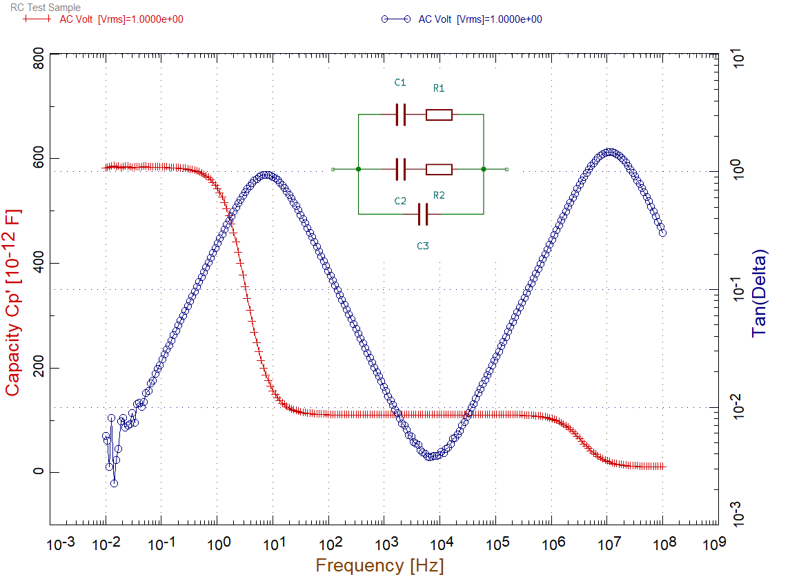
RC Network Sample
The sample consists of three capacitors and two resistors (all SMD parts) in the configuration:
(R1+C1)|(R2+C2)|C3 (+ for serial, | for parallel configurations, respectively).
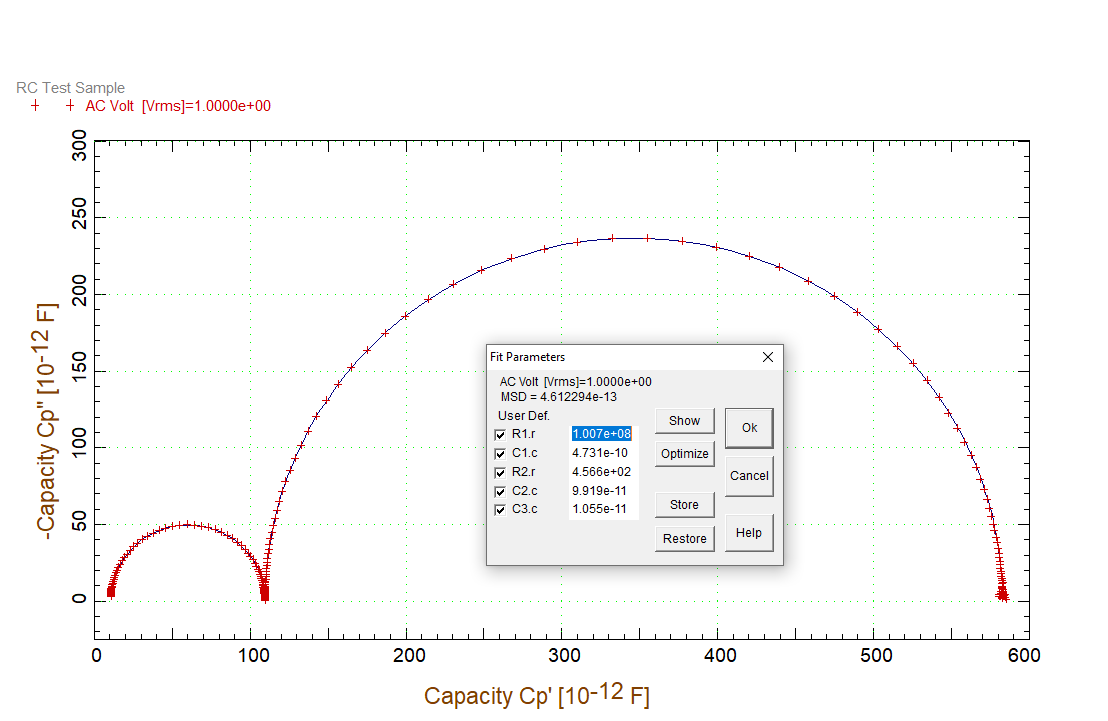
NEISYS RC Network Measurement.
R1/Ω
C1/F
R2/Ω
C2/F
C3/F
1.007 M
473.1 p
456.6
99.19 p
10.55 p
NEISYS RC Network Measurement up to 100 MHz. Inset: Fitted parameters.
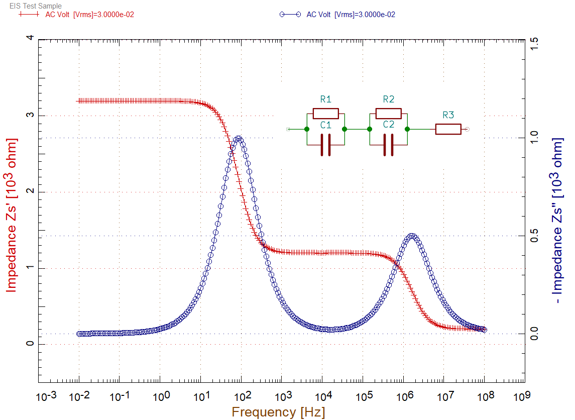
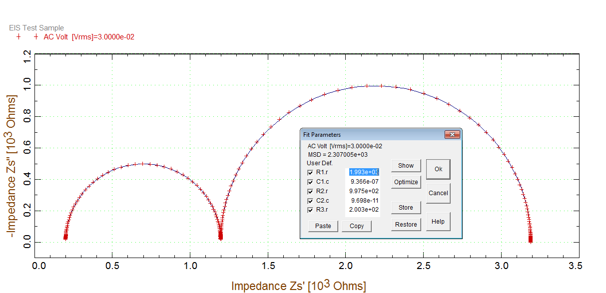
EIS Test Sample
NEISYS RC Network Measurement up to 100 MHz. Inset: Fitted parameters.
Configuration: (R1|C1)+(R2|C2)+R3
R1/Ω
C1/F
R2/Ω
C2/F
R3/Ω
1.993 k
0.9366 µ
997.5
96.98 p
200.3
NEISYS RC Network Measurement up to 100 MHz. Inset: Fitted parameters.
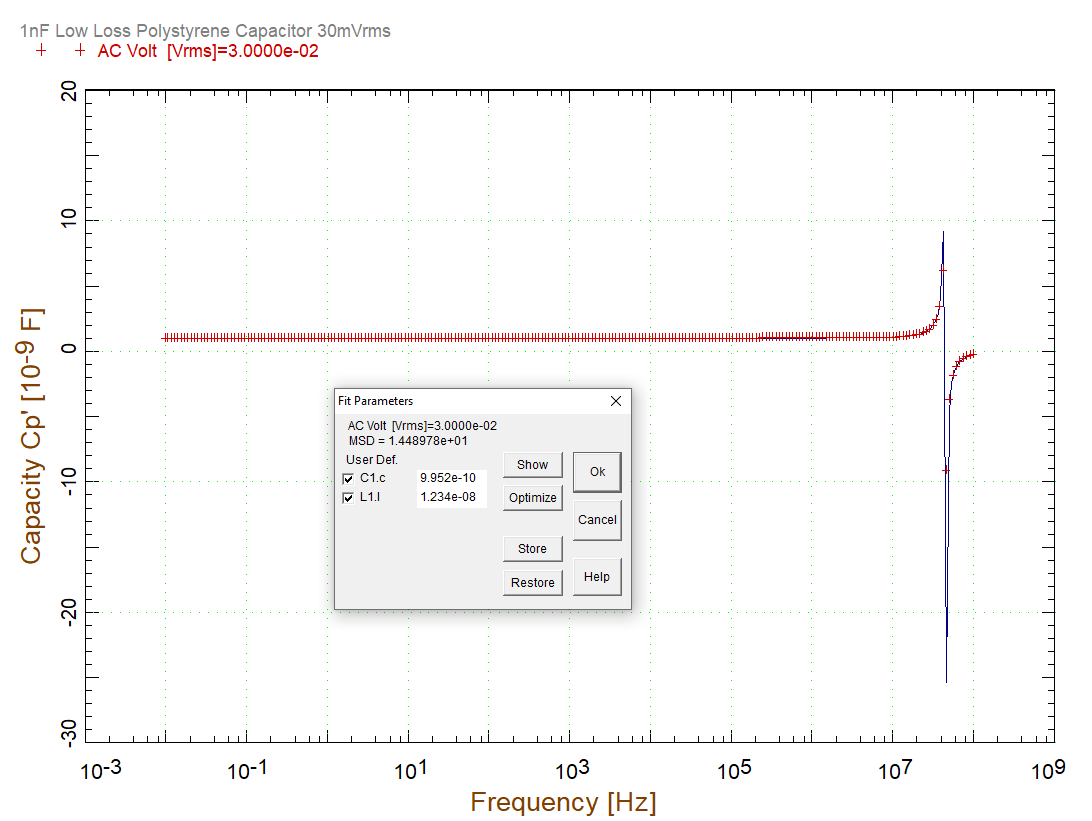
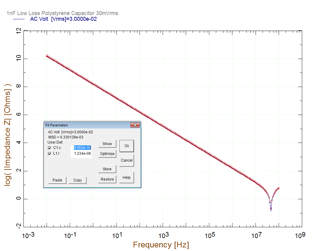
Capacitor 1 nF
Fit model: C1+L1
C1/F
L1/H
0.9952 n
12.34 n
NEISYS measurement of a 1 nF capacitor up to 100 MHz. Inset: Fitted parameters. NEISYS measurement of a 1 nF capacitor up to 100 MHz. Inset: Fitted parameters.
The plots show the measurement result for a 1 nF capacitor. The model for the fit is a simple serial configuration of
the capacitor with an inductance, C1 + L1. The fit delivers a capacitance of 0.9952 nF and a tiny inductive contribution
of 12.3 nH. Such inductance roughly corresponds to a single wire of 0.5 mm diameter and 10 mm (!) length.
This example illustrates that even a very short extra connection wire may easily contribute drastic effects in the
frequency range above 1 MHz, even if decent calibrations are used. Great care must be taken that the lengths of leads in
the circuit are maintained as exactly as possible between calibration and sample measurements. In the case above, we see
a resonance at about 45 MHz.
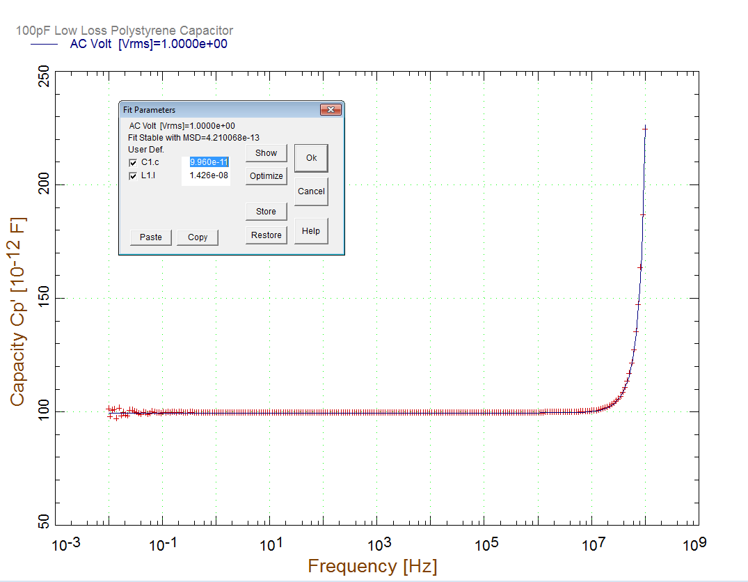
Low-Loss Test Capacitor 100 pF
Fit model: C1+L1
C1/F
L1/H
99.6 p
14.3 n
NEISYS measurement of a 100 pF capacitor up to 100 MHz. Inset: Fitted parameters.
The plot shows the measurement result for a low-loss 100 pF capacitor. The model for the fit is a simple serial
configuration of
the capacitor with an inductance, C1 + L1. The fit delivers a capacitance of 99.6 pF and a tiny inductive contribution
of 14.3 nH. Such inductance corresponds to a single wire of 0.5 mm diameter and about 10 mm (!) length.
While we do not see the full resonance in this case (which would appear at about 133 MHz), we can still see the
strongly
rising measured capacitance in this case which is due to the relatively small inductance of 14.3 nH.
Note: the rise of capacitance is not a deficiency of the instrument but the strong effect of a relatively
tiny inductance contribution. The visibility of such effects depends on the impedance contribution of the sample
itself.
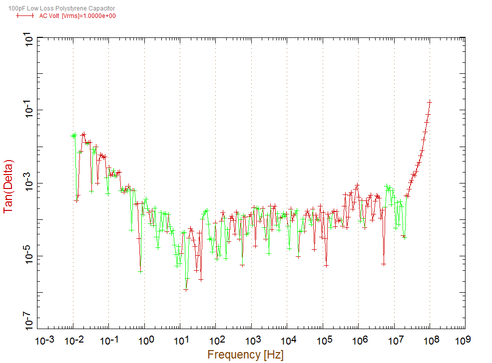
The following figure shows the loss factor measurement results of the same sample.
NEISYS measurement: Loss factor (noise floor) of a 100 pF low-loss capacitor up to 100 MHz.
Green color signals negative loss values.
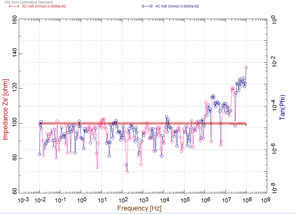
100 Ω Calibration Standard
NEISYS measurement of an 100 Ohm calibration standard. Tan(φ) in magenta indicate values below zero.
The measurement of the 100 Ω calibration resistor emphasizes the quality of the calibration procedure yielding decent
results up to the maximum frequency of 100 MHz. Also shown is tan(φ) showing values close to zero as expected for a test
object with strongly ohmic character.
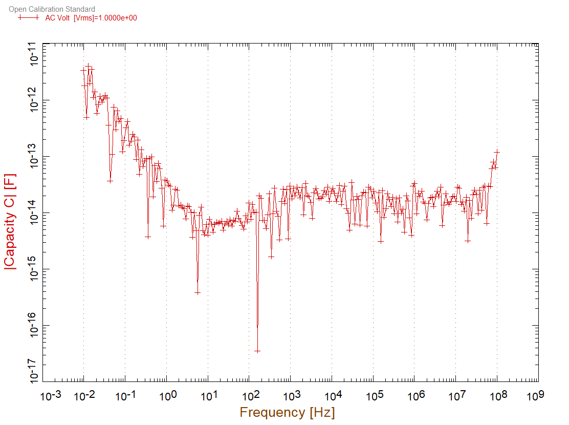
Open Calibration Standard
NEISYS measurement of an open calibration standard.